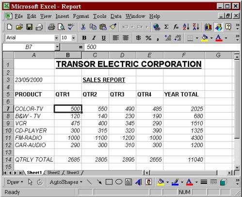
5.9 Efficient data display with data formatting

Formatting makes the data clear, understandable and presentable. By formatting your data you can also integrate your worksheet with an existing presentation or report. The tools offered for this purpose by Excel are: AutoFormat, Format printer and the buttons on the formatting.

Before we start create a worksheet as shown in picture and save it as REPORT.xls.

5.9.1 Formatting Data Automatically

5.9.1.1 Steps to format data with AutoFormat

1.    Open REPORT.xls.

2.    As a first step, select the range A5:A12.

3.    Next on the Format menu, click AutoFormat.

4.   In this dialog box you will see a table format: list. Scroll downward in the list, select 3D Effects2, and  then click OK. You will see that your data gets formatted in the 3D Effects2 style.

Click anywhere to have a clear view. You’ll notice that the worksheet table has shrinked from its original size.

5.    Close the worksheet without closing.

6.    Open the file once again.

7.    Before proceeding further, add a row at A15 by selecting A15:A16 and clicking on Insert men – Row option. Type Total and press enter.

 5.9.1.2 Format Data With Another Option

1.    Again select range A5:F12.

2.    On the Format Menu, click AutoFormat. The AutoFormat dialog box opens.

3.    In Table format: list, select Classic 3 and click the options >> Button. The AutoFormat dialog box expands to display the formatting options.

4.    Next in the formats to apply box, click the Number and Width/Height check boxes. Clearing the check marks from these boxes turns of these AutoFormat attributes and ensures that the number formats, column widths and row heights in each cell remain as they are in the original worksheet.

5.   Click on the OK button. The AutoFormat dialog box closes and the changes take effect.

Take a note that the worksheet table has not shrinked from its original size this time.

5.9.1.3 Repeat Auto Formatting.

In this section we will discuss how to apply the formatting (which we have just applied to a part of worksheet) to other parts of the worksheet. We will try to apply the format applied to A5:A12 to the range A16:B19.

1.    Select A16:B19.

2.    On the Edit menu, click Repeat AutoFormat. (Note: - that if you perform any other activity after applying AutoFormat, the option of Repeat AutoFormat will not be available for use.)

5.9.2 Copying Formats to Other Cells

If you wish to copy the formatting used in one section of your worksheet to another, you can use Format Printer button. This button allows you to copy format quickly. Lets find out the how to do it:

1.    Select row number 6. Right click and select Delete. The row gets deleted.

2.    Keep the cell pointer on cell A13 and click on cell A13 and click on the Insert menu, select rows. One blank row gets inserted.

3.    In cell B13, type the title QT1-TOT, in cell C13 type QT2-TOT, in cell D13 type QT3-TOT, in cell E13 type QT4-TOT and finally in cell F13 type Year Total. 

5.9.2.1 Copy A Format With The Format Painter Button

1.   Select the range A5:F6. On the Toolbar, click the Format Printer button. The pointer changes to a paintbrush with a plus sign.

2.    With this new pointer, select cell A13. The formatting is copied to range A13:F14.

Copyright © 2001 Selfonline-Education. All rights reserved.